This tutorial is intended to demonstrate how to use MATLAB tools to extend the functionality of MicrobeTracker. A typical problem in the analysis of microscope images is identification of large intracellular objects, such as protein filaments, nucleoids, injected particles, or protein aggregates. When big enough, these objects are very different from nearly diffraction-limited spots and therefore require special treatment. The desired propertis could be their number, size (area on an image), total intensity, or centroid location. This tutorial demonstrates how to use standard MATLAB functions perform (including some of the functions of the Image Processing and Mapping toolboxes) in order to perform some of the mentioned tasks and to provide a framework for the others.

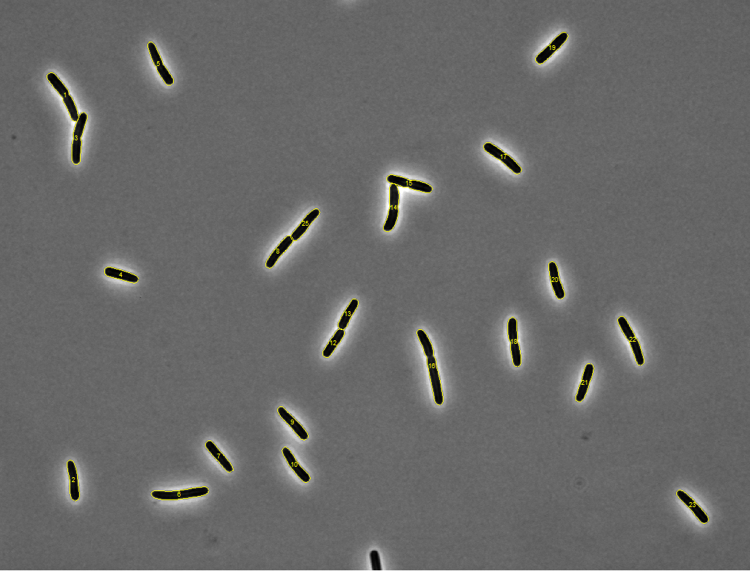
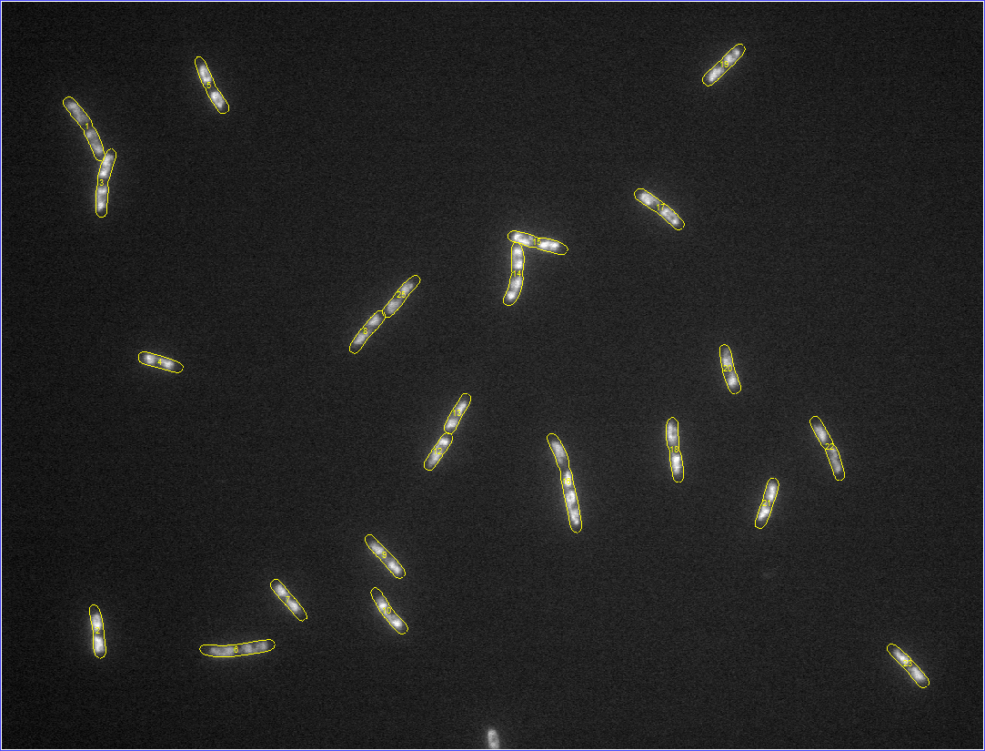
The image set for this tutorial is of E. coli cells grown in M9 media expressing HU-CFP and imaged in phase contrast and fluorescence modes on an agarose pad, so that their nucleoids are visible (courtesy of Dr. Manuel Campos, Jacobs-Wagner lab). The tutorials shows how to count the number of nucleoids per cell, calculate their total and relative areas, as well as the fluorescence intensity.

The data for the tutorials is not available by default. Please, make sure you download the version of the MicrobeTracker Suite "with examples" from the MicrobeTracker website.

The tutorial is divided into two sections: Pixel-based processing and Subpixel-resolution processing. The first one provides an easier mode of analysis, sufficient in most cases. The second one uses some advanced Mapping toolbox functions and is helpful when high precision is required or the cells and intracellular objects are only a few pixels in size.

The tutorial assumes that the cell meshes are already obtained, they are available in the meshes.mat file in the microbetracker_nucleoid subfolder. This subfolder also contains the phase contrast image used to generate the meshes (phase.tif) and the fluorescence image used in this tutorial to calculate the signal (fluo.tif). The tutorial assumes that the user knows how to load the meshes into the MATLAB workspace and how to run the included scripts. It is also recommended for the user to be familiar with the basics of the Image Processing toolbox, which can be achieved by going through the Getting Started tutorials on MATLAB's website. For reference, the images with detected meshes are shown below (click on an image to see a zoomed version).

Pixel-based processing

1. Load the meshes and the fluorescence image into the MATLAB workspace.

   load('meshes.mat','cellList')
   image = loadimagestack('fluo.tif');

Here MicrobeTracker's loadimagestack function is used, capable of loading multiple images. To load a single image, MATLAB's imread function can be used instead.

2. Images in MATLAB can be stored either as arrays of unsigned integers or as doubles. By default, a loaded image will be in the unsigned integer format at the precision of the number matching that of the image file. Many processing functions, however, require the image in double format, which takes more space. When processing stacks of images, it is recommended to convert them to doubles only one image at a time to save memory:

   image = im2double(image);

3. Let's perform processing for the cell #2 in the dataset. The dataset contains one frames, therefore the frame number will be 1. To reduce the amount of text to write, get the variables for this particular cell we need: the "box" identifying the area of the image containing the cell, and the mesh of the cell (see Output Format section for a description of these variables):

   box = cellList{1}{2}.box;
   mesh = cellList{1}{2}.mesh;

4. Crop the fluorescence image around the cell using imcrop function:

   img1 = imcrop(image,box);

And convert the meshes to the cropped image coordinates:

   mesh(:,[1 3]) = mesh(:,[1 3])-box(1)+1;
   mesh(:,[2 4]) = mesh(:,[2 4])-box(2)+1;

5. Display the image and the mesh outline:

   imshow(img1,[]);
   hold on
   plot(mesh(:,1),mesh(:,2),'y',mesh(:,3),mesh(:,4),'y')
   set(gca,'position',[0 0 1 1])

Here the second argument of imshow function ([]) means automatic scaling of the image. In the second line, hold on is used to retain the image when the outline if drawn. The last line uses set command to change the axes position and expand the image in the figure.

6. Convert the mesh to a polygon in order to use MATLAB's commands operating with this format. The polygon consists of two variables - x and y coordinates of the points on the outline of the cell:

   x0 = [mesh(:,1);flipud(mesh(1:end-1,3))];
   y0 = [mesh(:,2);flipud(mesh(1:end-1,4))];

7. Here is one example of using the polygon. Produce a mask of the cell using poly2mask command - a binary image with 1's corresponding to the pixels inside the cell and 0's to the pixels outside:

   cellmask = poly2mask(x0,y0,box(4)+1,box(3)+1);

8. The next step is to identify the nucleoid. One way to distinguish the nucleoid (or another object) from the background is to find a threshold intensity such that the regions of higher intensity would correspond to the nucleoid, and the objects of lower intensity to the background. For this MATLAB's graythresh function can be used. To use this function, first normalize the image to span the range of intensities from 0 to 1, since othervise it may fail:

   img2 = img1-min(img1(:));
   img2 = img2/max(img2(:));

And then run graythresh function. Here only the pixels inside the cell are used to calculate the threshold, they are obtained by using the cell mask as an index for the image variable, i.e. img2(cellmask):

   g = graythresh(img2(cellmask));

To get a mask corresponding to the nucleoid, get all the points with intensities above the threshold:

   nucleoidmask = img2>g;

There are alternatives to graythresh function to find objects in an image. One popular alternative is applying a "Mexican hat" fitler to the image in order to enhance the boundaries (use MATLAB's fspecial command with 'log' parameter to create the filter and imfilter to filter the image), and then take the areas below zero (sometimes below a different threshold). This approach is beneficial when the object is assumed to be of about uniform intensity and to have sharp boundaries, corrupted by diffraction. In such case enhancing the boundaries is meaningful. In the case of a nucleoid, where DNA density may decay very gradually, using boundary-enhancing filters may result in rejection of weak areas neighboring brighter areas of the nucleoid. In such cases, simple thresholding is prefered and therefore it was chosen here.

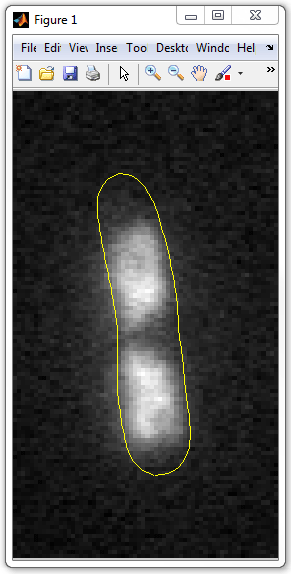
9. Let's now visualize the nucleoid. For this use imshow command as before. We'll combine the cell and the nucleoid masks to make the nucleoid white on gray background of the cell and black background outside.

   imshow(cellmask*0.5+nucleoidmask*0.5)

To display the cell outline, use the "hold on" command first, and then visualize the outline polygon:

   hold on
   plot(x0,y0,'y')

10. Now let's cycle through all the cells in this example visualizing the nucleoids in them. For this, open in the editor the script get_nucleoid_pixilated_vis.m provided with this example. I.e. type:

   edit get_nucleoid_pixilated_vis

And then set a breakpoint in line 27 by clicking the dash after the line number. After that, run the script by clicking Run button:

The script will display a cell and stop at the breakpoint. To continue to the next cell, click Continue button or press F5.

11. Let's now calculate the number of nucleoids per cell. For this, use MATLAB's regionprops function to identify discontinuous regions in the nucleoid mask:

   regstats = regionprops(nucleoidmask);

Then cycle through all regions picking those with the area larger than some prefixed area areamin. On each step, if the region is large enough, the counter nucleoidcount is incremented:

   areamin = 50;
   nucleoidcount = 0;
   for i=1:length(regstats)
       if regstats(i).Area>=areamin
           nucleoidcount = nucleoidcount+1;
       end
   end
   nucleoidcount

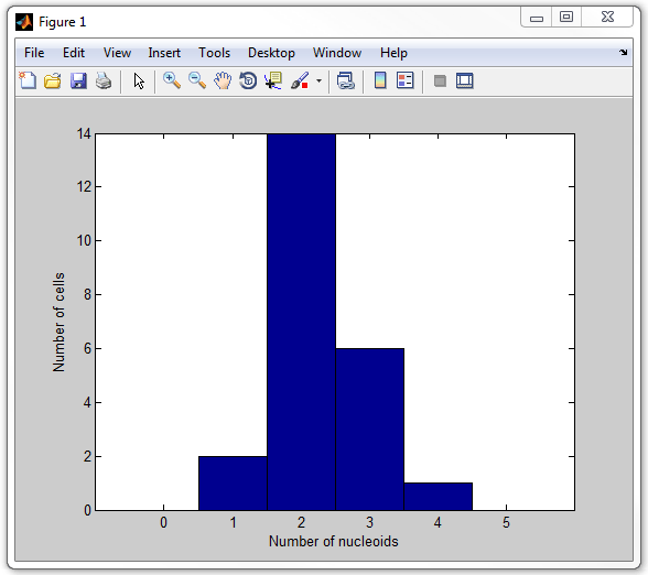
A script that cycles through each cell, calculates the number of nucleoids, and then displays a histogran of the number of nucleoids per cell is provided with this example and is called get_nucleoid_count_pixilated.m. Now run it:

   get_nucleoid_count_pixilated

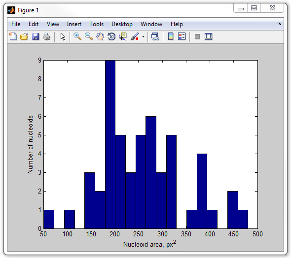
12. Let's now calculate the nucleoid areas. With a small modification of the above script, we now append the areas of the nucleoids we were counting before:

   nucleoidareaarray = [];

   areamin = 50;
   for i=1:length(regstats)
       if regstats(i).Area>=areamin
           nucleoidareaarray = [nucleoidareaarray regstats(i).Area];
       end
   end

Here is another script provided with the example that displays a histogram of nucleoid areas:

   get_nucleoid_area_pixilated

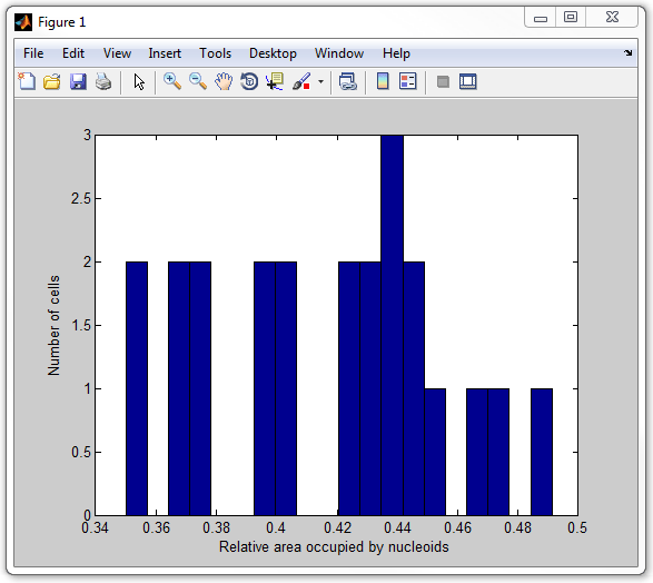
13. Now, let's calculate the fraction of the cell occupied by nucleoids. This time we don't need the regoinprops function. We calculate the areas of both the cell and the nucleoid as sums of pixel values for the masks, as the masks have value 0 for the pixels outside and 1 for the pixels inside the object:

   cellarea = sum(cellmask(:));
   nucleoidarea = sum(nucleoidmask(:));

To get a fraction, simply divide one by the other:

   nucleoidarea/cellarea

Another script provided with the example displays a histogram of the relative areas occupied by nucleoids:

   get_nucleoid_relative_area_pixilated

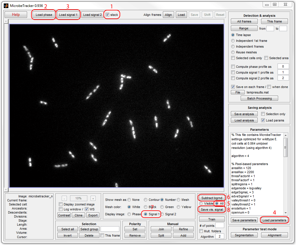
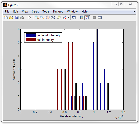
14. Finally, let's calculate the average intensity of the signal inside cells and inside nucleoids for every cell, and display as two histograms. For this, an extra step of removing the background from the fluorescence image is required. Run MicrobeTracker, load phase contrast and fluorescence images, load parameters, select All radio button on the Background subtraction panel and click Subtract bgrnd, then click Save vis. signal and save the buckground-subtreacted fluorescence image to a new file (here fluo_subtracted.tif was used). See the image below for a sequence of operations in MicrobeTracker:

To calculate the total signal in the nucleoid sum the image pixels in the mask:

   sum(img1(nucleoidmask))

And divide them by the total area, i.e. for the nucleoids and for the cells:

   nucleoidint = sum(img1(nucleoidmask))/sum(nucleoidmask(:));
   cellint = sum(img1(cellmask))/sum(cellmask(:));

The rest of the procedure is similar to the procedures described above. The whole script calculating the intensities (total signal divided by the area) in nucleoids and in the cells (including nucleoids) is called get_nucleoid_intensities_pixilated.m. Now execute it:

   get_nucleoid_intensities_pixilated

Subpixel-resolution processing

1. The beginning of subpixel-resolution processing is the same up to the point of determining the threshold. I.e. for cell #1 on frame #1:

   load('meshes.mat','cellList')
   image = im2double(loadimagestack('fluo.tif'));
   box = cellList{1}{1}.box;
   mesh = cellList{1}{1}.mesh;
   x0 = [mesh(:,1);flipud(mesh(1:end-1,3))]-box(1)+1;
   y0 = [mesh(:,2);flipud(mesh(1:end-1,4))]-box(2)+1;
   img1 = imcrop(image,box);
   mask = poly2mask(x0,y0,box(4)+1,box(3)+1);
   img2 = img1-min(img1(:));
   img2 = img2/max(img2(:));
   g = graythresh(img2(mask));

2. Then we find the outline of the nucleois or nucleoids in the cell. First, set the value of the pixels outside of the cell to zero so that no objects are detected outside. However, a fraction of a pixel may be inside of the cell even though its center is outside. Therefore, we first expand the cell mask by one pixel outwards:

   expandedmask = imdilate(mask,strel('square',3));

And then set the values of the outside pixels to zero (the ~ sign means negation):

   img2(~expandedmask)=0;

Now we can determine the contours at subpixel resolution by using MATLAB's contourf function. This function uses linear interpolation between pixels to get the outline as precise as the information in the image allows, not limited to the pixel size:

   c = contourf(img2,[g g]);

The format of the output will be explained below.

2. Now lets parse the contour structure obtained with the contourf command. The structure consists of the lines of x and y coordinates of individual contours, separated by the values of the polygons (equal to g here) and the number of vertices in each polygon. See contour matrix description for details. To parse the structure, we can go through, extracting the individual polygons (with coordinates of the vertices x and y) on the way:

   ind = 1;
   while ind<size(c,2)
       ctr = c(:,ind+1:ind+c(2,ind))';
       ind = ind+c(2,ind)+1;
       x1 = ctr(:,1);
       y1 = ctr(:,2);
   end

3. In order to take only the portions of the polygons inclosed in the cell outline, we can use MATLAB's polybool function:

   [x2,y2] = polybool('intersection',x0,y0,x1,y1);

Note that polybool function assumes that the contours have clockwise orientation, and though it works, it displays a warning otherwise. To convert counterclockwise-oriented contours to clockwise orientation, use MATLAB's poly2cw function (this step is not shown here, but included in the final script).

Let's display the (x1,y1) and (x2,y2) polygons to see what we achieved so far. Copy and paste the code below to MATLAB's command window (assuming the contour c-structure has been already generated). The cell outline will be plotted in yellow color, the original polygons in green, and their portions inside the cell in red:

   figure
   imshow(img1,[])
   set(gca,'pos',[0 0 1 1])
   hold on
   plot(x0,y0,'y')
   ind = 1;
   while ind<size(c,2)
       ctr = c(:,ind+1:ind+c(2,ind))';
       ind = ind+c(2,ind)+1;
       x1 = ctr(:,1);
       y1 = ctr(:,2);
       [x2,y2] = polybool('intersection',x0,y0,x1,y1);
       plot(x1,y1,'g')
       plot(x2,y2,'r')
   end

4. Now separate the outlines of the nucleoids from the outlines of the included empty areas. This can be done by determining the orientation of the polygons included in the contour c-structure: the outer polygons will have clockwise orientation, while the internal ones - counterclockwise. To determine the orientation or a polygon, MATLAB's ispolycw function can be used (or a faster MicrobeTracker's isContourClockwise function).

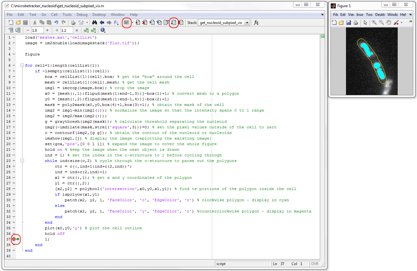
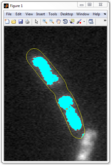
Run included get_nucleoid_subpixel_vis.m script in debug mode to visualize the nucleoids in every cell one-by-one. For this, open the script in the editor, put a breakpoint in line 38, and run the script. The nucleoids will be shown as cyan patches, the "holes" in them will be colored yellow.

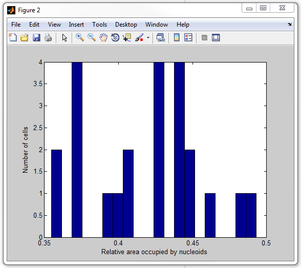
5. Finally, let's calculate the relative areas occupied by nucleoids. For this, go through the nucleoid regions and add the areas of those with clockwise orientation (external), substracting those with counterclockwise orientation (internal):

   cellarea = polyarea(x0,y0);
   nucleoidarea = 0;
   ind = 1;
   while ind<size(c,2)
       ctr = c(:,ind+1:ind+c(2,ind))';
       ind = ind+c(2,ind)+1;
       x1 = ctr(:,1);
       y1 = ctr(:,2);
       [x2,y2] = polybool('intersection',x0,y0,x1,y1);
       if ispolycw(x1,y1)
            nucleoidarea = nucleoidarea+polyarea(x2,y2);
       else
            nucleoidarea = nucleoidarea-polyarea(x2,y2);
       end
   end

The relative area will be a ratio of nucleoidarea to cellarea:

   nucleoidarea/cellarea

The whole script calculating this ratio for every cell and displaying it in for of a hystogram is called get_nucleoid_relative_area_subpixel.m. Now execute it:

   get_nucleoid_relative_area_subpixel

It is not difficult to get individual nucleoid areas. However, the problem of precisely integrating the signal inside arbitrary polygons is significantly more challenging. Those who are interested can refer to getOneSignalC function in MicrobeTracker's code itself.