This tutorial is intended to demonstrate the steps in using MicrobeTracker to detect E. coli cells on a single image, as well as to demonstrate some basic tools for cell shape analysis. For a more general description of the cell detection procedure, the other steps of MicrobeTracker operation, and the full list of tutorials see Quick Start section of the help. This tutorial assumes that the installation procedure has been already performed as described.

The data for this tutorial is not available by default because of its large size (about 10 MB). Please, make sure you download the version of MicrobeTracker that contains all tutorials from the MicrobeTracker website.

1. Start MATLAB. Set the working path in MATLAB to the folder of the example: .../MicrobeTracker.../examples\microbetracker_ecoli (see the image below, click on the image for its full resolution version).

2. Type microbeTracker in MATLAB's command window to start MicrobeTracker. A new MicrobeTracker window will open.

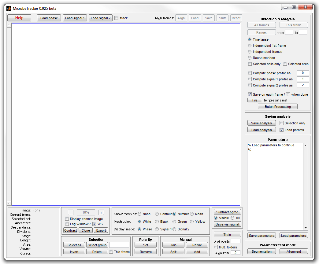
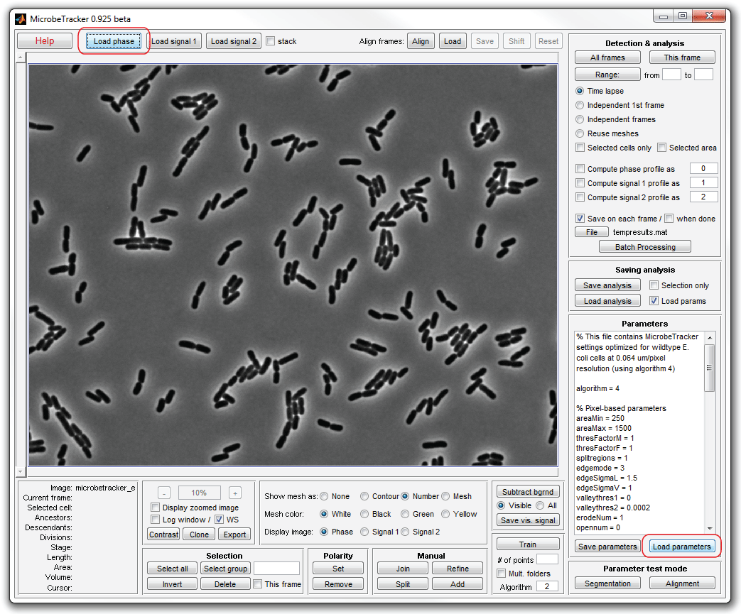
3. Click Load phase and select the phase_contrast subfolder of the example folder to load the images. Click Load parameters, browse to the example folder and select the alg4ecoli3.set file to load the parameter set best adjusted for this image type.

4. Now perform cell detection. To do that, click This frame and wait for the program to detect all cells. It will take several munutes, during which the program will display some information abut the processing in the MATLAB workspace window. When it finishes, the detected cells will be displayed with their numbers.

5. In order to see the cells better, select Contour and Green on the Objects to display panel in the bottom.

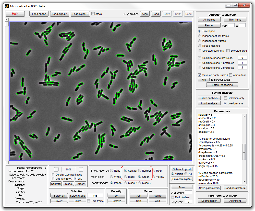
6. Make manual corrections to the occasional errors in cell detection. Use a zoomed image (called by selecting Display zoomed image checkbox) to display cells at higher resolution. Use mouse wheel or - and + buttons on the Zoom panel to zoon in and out.

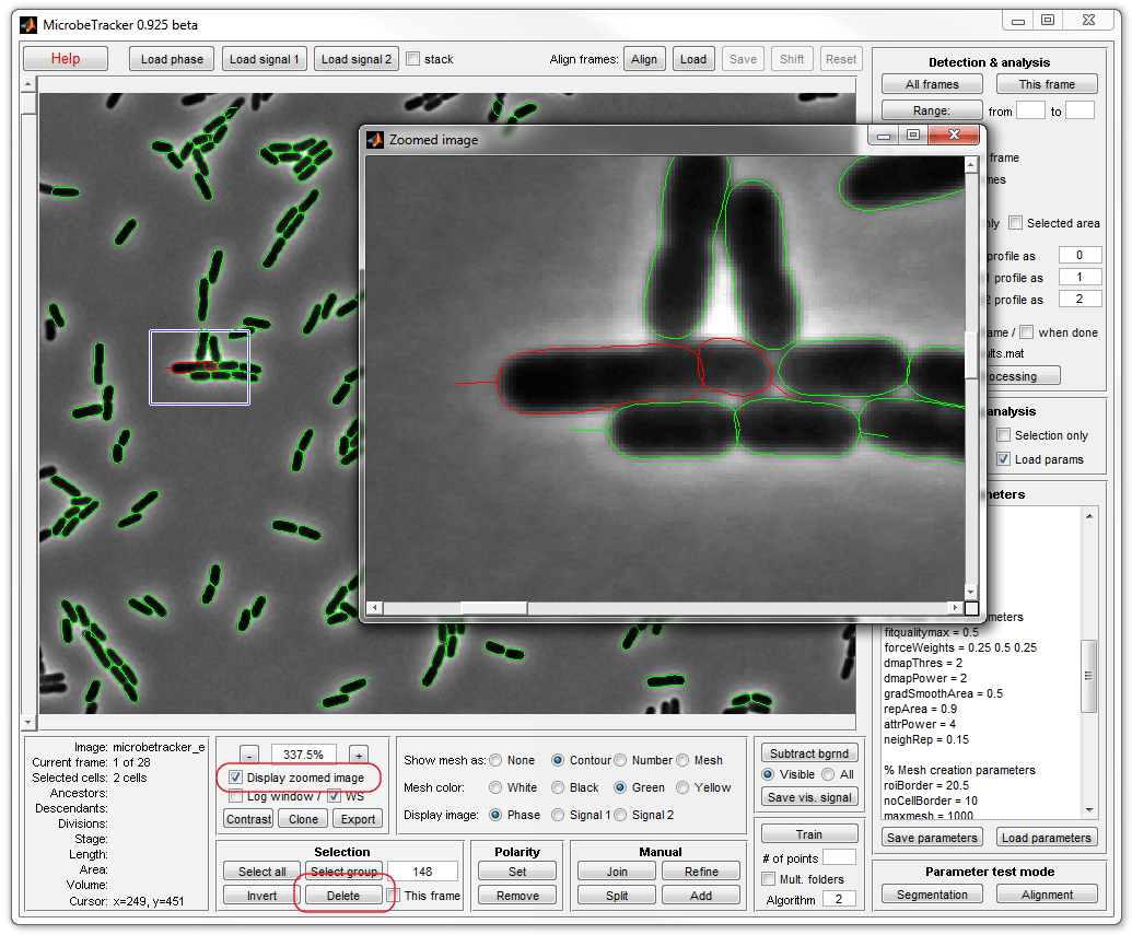
7. To join two cells (in the image) select those cells by clicking on them either in the main or in the zoomed window while holding the keyboard SHIFT button (to select more than one cell) and click Join on the Manual panel.

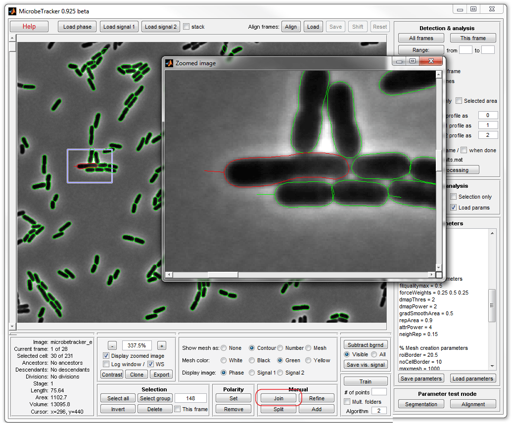
8. Finish joining and removing cells (by clicking Delete). Now you can save the results of your analysis by clicking Save analysis button (a file is already provided with MicrobeTracker, so you can skip this step this time).

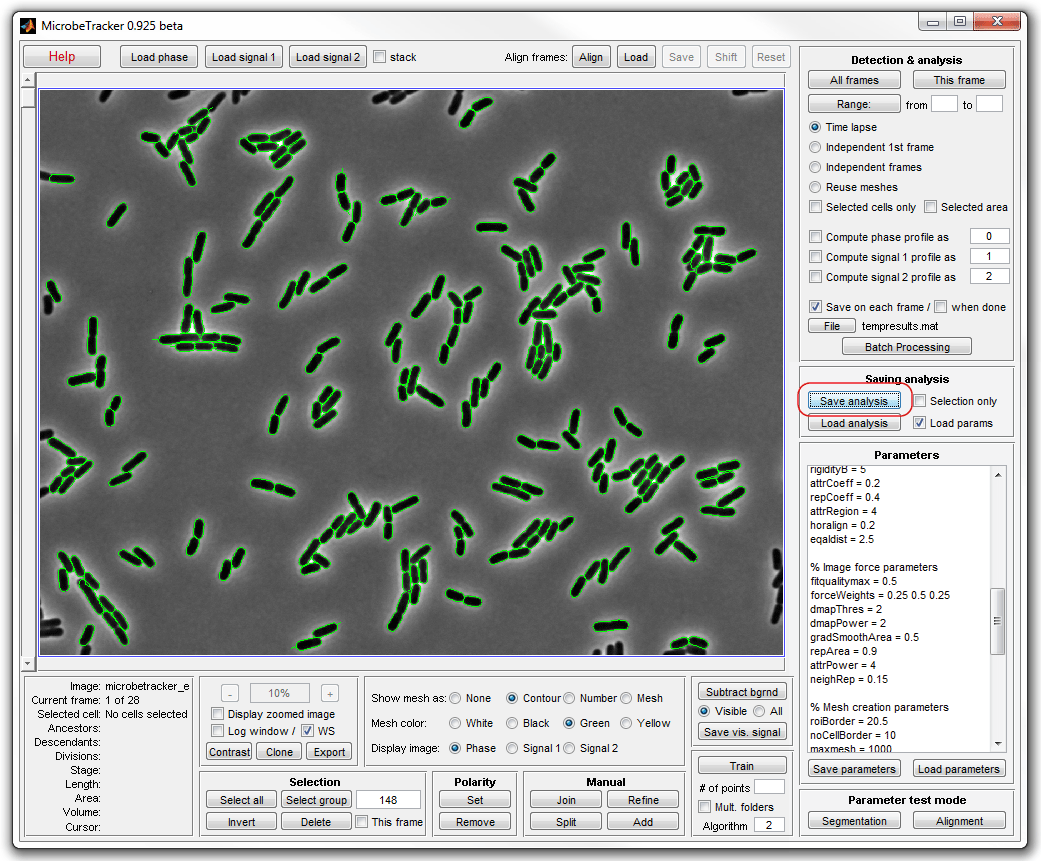
9. In what follows, the tutorial demonstrates what information can be extracted from the data we just obtained. Close microbeTracker and load the meshes from the saved file into MATLAB command window either by dragging and dropping or by typing (the information that you type will be indicated by MATLAB invitation >>:

   >> load('meshes')

10. Now a few new variables appear in MATLAB's workspace subwindow, the most important being cellList. Display some basic statiscs on the experiment by typing:

   >> cellstat(cellList)

Total number of cells: 229, located on 1 frames
Total number of spots: 0, located in 1 cells (0 spots/cell)
Cell length is 43.8474 +/- 10.3947 pixels (mean +/- st. dev.)
Cell width is 14.0543 +/- 0.82771 pixels
Cell area is 620.3603 +/- 168.4189 pixels^2
Cell volume is 7296.4757 +/- 2196.6474 pixels^3

11. Display a histogram of cell length by typing (make sure the MicrobeTracker window is closed, otherwise the command will plot into that window; reload the meshes after you close the window):

   >> lengthhist(cellList)

Cell length, pixels
Processed 1 dataset
Set 1: mean 43.8474, std 10.3947

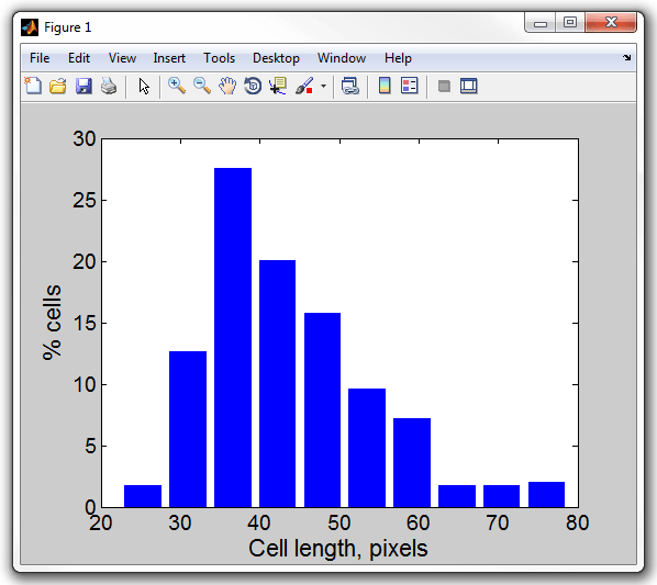
12. Notice that the length of the cell is indicated in pixals because MicrobeTracker does not know about the actual recolution of the microscope. To display the same histogram in microns enter the conversion factor, which is in this case 0.0652 µm/pixel:

   >> lengthhist(cellList,0.0642)

Cell length, um
Processed 1 dataset
Set 1: mean 2.815, std 0.66734

13. Display a histogram of the mean width of the cells (i.e. everaged for each cell across the length of its body). Notice, in the previous example the figure window was replaced. Open the results in a new window this time:

   >> figure
   >> meanwidthhist(cellList,0.0642)

Mean cell width, um
Processed 1 dataset
Set 1: mean 0.87521, std 0.054137

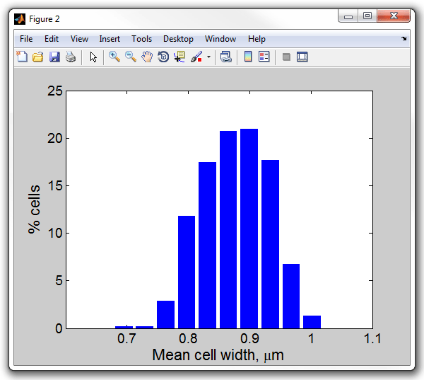
14. In order to save the width of each cell in MS Excel format to process in a different application type (assiming you have MS Excel installed on your computer):

   >> mwanwidthlist = meanwidthhist(cellList,0.0642)
   >> xlswrite('xlsdata',mwanwidthlist')

In this example the apostroph after the mwanwidthlist variable transposes the matrix to write it as a column rather than as a row. Notice that a file named xlsdata.xls appeared in the example folder. If you open this file in Excel, you will see that the first column contains the information about the mean width (in microns) of each of the 229 cells in the image.